Randomized term grouping over physical law on digital quantum simulation
Advisor: Dr.Alex Thom (Yusuf Hamied Department of Chemistry)
Introduction
One of the advantage of quantum computing over classical computation is to simulate complex quantum systems. This idea was originally proposed famously by Richard Feynman[1]:
“Let the computer itself be built of quantum mechanical elements which obey quantum mechanical laws.”
In the past few decades, various algorithms have been put forward. Seth Llodys[2] first formulated the problem for local Hamiltonian simulation where k-local means, for $H = \sum_j^{L} H_j$, each term acts on at most k qubits rather than all n qubits. In this case the problem is reduced to polynomial space: $L = \text{poly}(n)$ since $L \leq \sum_{j=1}^{k} {n \choose j} \leq c {n \choose j} \leq \frac{n^{n-c}}{(c-1)!}$ with $L = \text{poly}(n)$. Given any Hamiltonian evolution unitary $U = e^{-iHt}$, we can find a set of quantum gates that could approximate the evolution: \[U \approx V = V_1 V_2 \dots V_N\]
He then explicitly used compilation method called product formula or trotterisation to find out how the error $\epsilon(U) = \Vert e^{-iHt} - V \Vert$, scales with system parameters: Consider many-body Hamiltonian as $H = \sum_{k=1}^{L} h_k H_k$, where $H_k$ is one sub-term (usually a Pauli string) in the Hamiltonian and $h_k$ is the associated coefficient. The first order trotterisation (or lie trotter) is defined as: \[S_1(t) = \prod_{k=1}^L \exp ( -i h_k H_k t)\]
the scaling follows as: \(N_t = \mathcal{O}(\frac{(t L \Lambda )^2}{\epsilon})\) where $\Lambda := \max_k \Vert h_k \Vert$. So to make better approximation we need to increase the time steps $N_t$: \[e^{-i\sum_{k=1}^{L} h_k H_k} \approx S_1(\frac{t}{N})^N = S_1(\delta t) S_1(\delta t) \dots S_1(\delta t)\]
Built upon that, higher order formula is derived for better scaling[3] in terms of Trotter errors but comes with a trade-off between number of gates required and precision per Trotter step and we can demonstrate that the balance is optimised around $2^{nd}$ and $4^{th}$ order. \[S_2(t) = \prod_{k=1}^L \exp ( -i h_k H_k \frac{t}{2})\prod_{k=L}^1 \exp ( -i h_k H_k \frac{t}{2})\]
\(S_{2k}(t) = S_{2k - 2}(p_kt)^2S_{2k - 2}\left( (1-4p_k)t\right)S_{2k - 2}(p_kt)^2\) where $p_k = 1/(4 - 4^{1/(2k - 1)})$ and they scale as: \(N = \mathcal{O}(\frac{(t L \Lambda )^{1+\frac{1}{2k}}}{\epsilon^{1/2k}})\)
The better accuracy comes from the fact that with recursive formula in both forward and backward direction some of the error terms in the non-commutativity will cancel out. More advanced techniques like linear combination of unitaries(LCU)[4], quantum signal processing[5] and truncated taylor series[6] have demonstrated improvements in different aspects afterwards. For example, with the truncation order for LCU the number of gates needed per step is approximately: \(\mathcal{K} = \mathcal{O}(\frac{log(\frac{1}{\epsilon})}{loglog(\frac{1}{\epsilon})})\)
while Trotterization has the exponential dependency, i.e. fourth-order $\mathcal{O}(\frac{1}{\epsilon^{1/4}})$. Not only does Taylor series give logarithmically better scaling, it also comes with a better empirical result7.
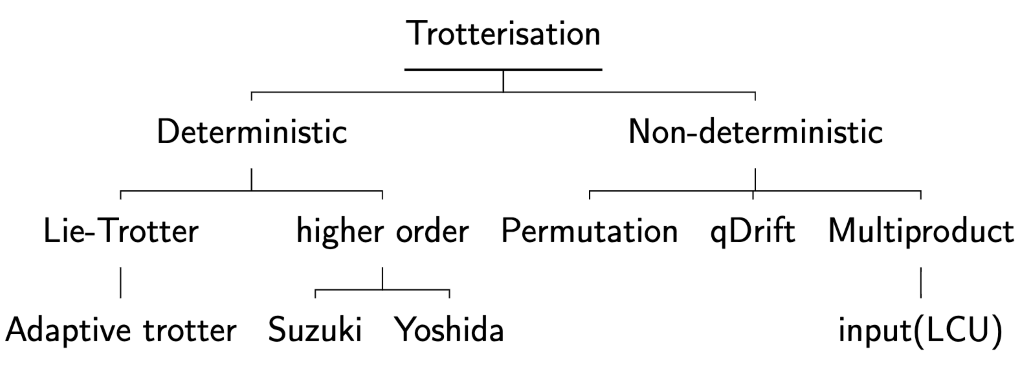
We mention alternative approaches briefly. Adaptive trotter[11] framework was recently proposed with better empirical error bound however this method involves feed-forwarding circuits and is not suitable for near-term application. Yoshida[12] used a leapfrog scheme for higher orders and it has been improved since[13]. With recent proposal on specific condition[14] to reduce the exponential parameter dependency in Multiproduct formula[4], the approach of parallelisation of product formula has become more practical.
But product formula remain to be the most popular one, particular for near-term hardware simulation[9,10]. This is because:
- Norm of the wavefunction is preserved: errors in expectation values are expected to oscillate, vs in non-unitary evolution errors accumulate, e.g. $| 1-iHt | \approx 1 + |H|t > 1$ with LCU.
- it has simple implmentation with no overhead (unitary operation can be implemented deterministically, without ancilla qubits)
However, despite achieving tighter error bound[7] for trotterisation and progress in tuning the parameter, e.g. $p_k$[15] to make simulation more accurate, problems remain with the intrinsic property of the algorithm: the exponential dependency of the recursive form $\mathcal{O}(5^k)$ and the inclusion of number of Hamiltonian terms L. The second issue is particularly prominent in large system like quantum chemistry where complex electronic structure involves a lot of Pauli strings after some transformation.
Consequently, several protocols focused on non-deterministic construction. In contrast to deterministic algorithms that produce unitary quantum circuits, randomized algorithms either randomly permute the ordering of unitary gates during simulation[16], which we will refer to ‘random permutation’, or utilize mixing lemma[17,18] on quantum channels (qDrift[19]) to make better asymptotic scaling. In this paper we will concentrate on these two major approaches and demonstrate the advantage of our algorithm by combining physical laws both theoretically and empirically. Specifically we show that simulating the evolution while preserving particle number makes the state-vector more accurate, which we refer as physDrift. We will show subsequently that this could be achieved by term grouping. Then deterministic methods are also included for benchmarking. We demonstrate that physDrift has smaller error and significantly reduces the leakage to unphysical system in both short and long time. That is to say, the conservation law is obeyed during evolution. Finally, to implement the circuits on real hardware we need to consider errors. So depolarising error is added and the simulation is again benchmarked for comparison.
Background
Hamiltonian evolution operator is hard to be directly implemented on quantum circuits. In this section we explain the method used to decompose and transform the unitary $e^{-iHt}$ and then integrate with near-term hardware.
Chemistry model
We focus on electronic structure problems, which could be initialized with electronic model (Molecular Hamiltonian or Fermi-Hubbard model in physics): \(H=\sum_{pq}h_{pq}a^\dagger_{p}a_{q}+\frac{1}{2}\sum_{pqrs}h_{pqrs}a^\dagger_{p}a^\dagger_{q}a_{r}a_{s}+h_{nuc}\)
where $h_{nuc}$ is the nuclear energy and we ignore it in the Born-Oppenheimer approximation, which makes it a constant. $a_p, a_p^\dag$ are fermionic operator satisfying: \(a^\dagger_1 \ket{0}_1 = \ket{1}_1,\quad a^\dagger_1 \ket{1}_1 = 0,\quad a_1 \ket{0}_1 = 0,\quad a_1 \ket{1}_1 = \ket{0}_1\)
and they anti-commute with operators with different labels. The coefficients are defined as: \(h_{pq} = \int_{-\infty}^\infty \psi^*_p(x_1) \left(-\frac{\nabla^2}{2} +V(x_1)\right) \psi_q(x_1)\mathrm{d}^3x_1\) \(h_{pqrs} = \int_{-\infty}^\infty \int_{-\infty}^\infty\psi_p^*(x_1)\psi_q^*(x_2) \left(\frac{1}{|x_1-x_2|} \right)\psi_r(x_2)\psi_s(x_1)\mathrm{d}^3x_1\mathrm{d}^3x_2\)
where $V(x)$ is the mean-field potential. In general $h_{pq}$ represents the integral contains kinetic energy + electron-nucleus attraction while $h_{pqrs}$ is the two-body interaction term. Together with the creation and annihilation operator, we can classify terms in Molecular Hamiltonian as in the following TABLE.
In particular, we have integrated $h_{pqpq}$ into $h_{pqqp}$. $h_{pqpq}$ is an exchange coupling - it’s only non-zero when the two electrons have the same spin so that they have antisymmetric spatial state which reduces the coulomb repulsion. So this term tends to induce ferromagnetic coupling between neighbouring spins. As we make the separation between sites bigger, the $h_{pqpq}$ term gets exponentially smaller we can consider only the $h_{pqqp}$ term. Correlated excitation between electrons means that the interaction depends on the location of the electrons, i.e. if electron 1 in r jumps to p, electron 2 in q stays in q. This can be seen directly from the expansion of the operator using fermionic anti-commutation relations:
\(a^\dagger_{p}a^\dagger_{q}a_{q}a_{r} = (a^\dagger_{p}a_{r} + a^\dagger_{r}a_{p})(a^\dagger_{q}a_{q})\) 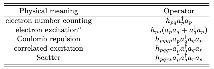
Transformation
Using the Jordan-wigner transformation[20], we can map fermionic operator to the space spanned by Pauli operators:
\(a^\dagger_j = \begin{bmatrix} 0 & 0 \\ 1 & 0 \end{bmatrix}=\frac{X_j - iY_j}{2}\) \(a_j= \begin{bmatrix} 0 & 1 \\ 0 & 0 \end{bmatrix}=\frac{X_j + iY_j}{2}\)
To given a concrete example, consider the excitation term: \(h_{pq}(a_p^\dagger a_q + a^\dagger_q a_p) = \frac{h_{pq}}{2}\left(\prod_{j=q+1}^{p-1} Z_j \right)\left( X_pX_q + Y_pY_q\right)\) Other mappings like Bravyi Kitaev transformation[21] and parity transformtion[22] are also available. But here we will stick to the simplest approach and leave improvements for future work.
Pauli gadgets
With Hamiltonian as Pauli strings in hand we consider the circuit below which is basically the controlled rotational gate in Z.
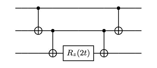
where the CNOT gates take the role as parity checker connecting all qubits together and the factor of 2 in the rotational gate comes from the fact that Pauli group, which belongs to SU(2), is actually a double cover of SO(3).
We just need to use the relation $HZH = X$ and $Y = (SH)Z(SH)^\dag$, where H is the Hadamard gate and S being the phase gate, to compute universal Pauli strings as below.
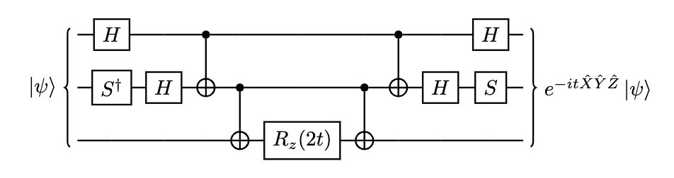
To simulate all Pauli strings we need to concatenate our circuits using following Theorem:
Theorem 1
For any two sub-terms $H_i$, $H_j$ in Hamiltonian $H = \sum_{k}^{L} h_k H_k$, if they satisfy, \([H_i, H_j] = 0\) then we have: \(e^{-i(H_i+H_j)t} = e^{-iH_it}e^{-iH_jt}\) *** So if the Pauli strings commute with one another, direct connecting Pauli gadgets together will give us the exact evolution operator. We also get the intuition that with more commutative terms, the error goes down. Bound has been proved through both commutator[7] and anti-commutator[23] relations.
Randomized protocols
In this section we begin by reviewing on density matrix: A classical distribution $p_i$ of quantum states gives a mixed state and must be described using a density matrix, \[\rho = \sum_{i=1}^{m} p_i \underbrace{\ket{i}}_{\text{pure state}} \bra{i}\]
If $m>1$, $\rho$ is a mixed density matrix. And we remind that for any $\rho$ the following properties are obeyed:
- $Tr(\rho) = 1$
- $\rho > 0$
- Hermitian
We also clarify some of the notations. All capital curly letter refer to the quantum channel, which correspondingly evolves density matrix by unitary operators, e.g. $\mathcal{U} = e^{iHt}\rho e^{-iHt}$. In the remaining paper we use $\mathcal{U}$ as the actual evolution channel and $\mathcal{V}, \mathcal{E}$ as approximations. We will sometimes utilize liouvillian representation for quantum channel: \[e^{iHt} \rho e^{-iHt} = e^{t\mathcal{L}} = \sum_{k=0}^\infty \frac{t^k \mathcal{L}^k (\rho)}{k!}\]
where \(\mathcal{L} (\rho) =i (H\rho - \rho H)\) And we have similarly as above the composition of Hamiltonians with sub-terms: \(\mathcal{L} (\rho) = \sum_{j} h_j \mathcal{L}_j\) \(\mathcal{L}_ j(\rho)=i(H_j\rho - \rho H_j)\)
A quantum channel describes how a particular state or more usefully, a mixture of quantum states evolves to another set of quantum states. The most general `channel’ is a CPTP(ompletely positive, trace preserving) map, i.e. something that maps a density matrix onto another density matrix: \(\rho \rightarrow \sum_i M_i^\dag \rho M_i, \text{ where $\sum_i M_i^\dag M_i = 1$}\) where $M_i$ is called Kraus operator\cite{Kraus}. Thus, classically sampling a series of exponentials defines a valid CPTP map with $M_i = \sqrt{p_i} U_i$: \(\rho \rightarrow \sum_i p_i U_i^\dag \rho U_i\)
If we start in a pure state, essentially we can generate the following mixed state: \(\ket{\psi}\bra{\psi} \rightarrow \sum_i p_i U_i^\dag \ket{\psi}\bra{\psi} U_i = \sum_i p_i \ket{\Psi_i}\bra{\Psi_i}\)
Metric
Now we introduce some useful result to help analysis of randomized algorithms. We use diamond norm to calculate the difference between simulated state-vector and actual one: \[d_\diamondsuit (\mathcal{E},\mathcal{U}) =\frac{1}{2} \Vert \mathcal{E} -\mathcal{U} \Vert_\diamondsuit = \sup_{\Vert \rho \Vert_1 =1} \frac{1}{2} \Vert ((\mathcal{E}-\mathcal{U}) \otimes \mathbb{I})(\rho )\Vert_1\]
where $\mathbb {I} $ is the identity channel which has the same size as $\mathcal{E}$ and $\Vert \cdot \Vert$ is Schatten-$1$ norm or trace norm. Trace norm can be basically considered as the Euclidean distance between two quantum states:
\(\Vert M \Vert = \operatorname {tr} (\sqrt{MM^\dag})\) \(M = \ket{\psi}\bra{\psi} -\ket{\phi}\bra{\phi}\) Following above we can show given an operator M, \(| \operatorname {tr} (M\mathcal{E}) - \operatorname {tr} (M\mathcal{U}) | \leq 2 \Vert M \Vert d_\diamondsuit (\mathcal{E},\mathcal{U})\) It’s important to note that because diamond norm evaluates the maximum possibility that the two channels can be distinguished in all quantum states(meaning that the smaller the value the closer the simulation is to reality), this is the worst scenario bound for measuring the error because effectively it is evaluating the error over all state vector space. Although other spectral error metrics have been assessed intensively[25], we still adapt diamond norm as it is the most commonly used ones in literature. As each quantum gate represents a unitary operator, to related it to quantum channel we employ mixing lemma:
Lemma 1
Let $\mathcal{U}=U\rho U^\dag$ and $\mathcal{V}j=V_j\rho V_j^\dag$ be unitary channels, and let ${p_j}$ be the probability distribution for the randomized protocol, suppose that: \(\Vert \sum_{j}(p_jV_j) - U\Vert \leq a\) Then the mixed channel $\mathcal{V}:=\sum{j}(p_j\mathcal{V_j})$ satisfy \(\Vert \mathcal{V} - \mathcal{U} \Vert \leq 2a\) ***
Note this is an improved version over the original lemma and the proof is in Appendix A\ref{apA} as well as [Lemma 3.4][26].
qDrift
With Lemma 1, we first choose an important sampling distribution ${p_j}$. Here we consider the original construction, i.e. $p_j = \frac{|h_j|}{\lambda}$ where $|\cdot|$ means absolute value and $\lambda = \sum_{j=1}^{L} |h_j|$ . More advanced important sampling technique could be used to reduce cost of the circuit[26,27]. Then for each sample step(qDrift does not have the idea of time step, instead it is number of Pauli strings sampled that specify the interval of evolution.) we sample from the pool ${H_j}$ and implement the Pauli string with modified coefficients $\lambda t / N$ with N being the total sample number. Effectively, with probability $\lambda^N \prod_{j=1}^N |h_{j_k}|$, we have constructed a quantum channel: \(\mathcal{V} = \prod_{k=1}^{N} \sum_{j=1}^L p_jV_j\rho V_j^\dag = \prod_{k=1}^{N} \sum_{j=1}^L p_je^{-i\lambda t/N H_j}\rho e^{i\lambda t/N H_j} = \prod_{k=1}^{N} \mathcal{V}_N = \prod_{k=1}^{N} \sum_{j=1}^L p_j e^{\tau\mathcal{L}_j}\)
the last one is in liouvillian form where $\tau = \frac{\lambda t}{N}$. To express it as unitary we can think of the expectation value of the resultant operator $\mathbb{E}[V_k] = e^{-it/N\mathbb{E}[h_k/p_k]}$ for a single mixed unitary and then for the whole process we have \[V = \mathbb{E}[V_N\dots V_1]\]
By telescoping lemma the scaling for qDrift as: \[N = \mathcal{O}(\frac{2(t \lambda )^2}{\epsilon})\]
Lemma 2 (Telescoping)
If $\mathbb{E}[V]$ and U are bounded by operator norm $\Vert \mathbb{E}[V] \Vert$, $\Vert U \Vert$ $\leq 1$, then: \(\Vert \mathbb{E}[V]^N - U^N \Vert \leq N\Vert \mathbb{E}[V] - U \Vert\) ***
It is worth noting that the number of gates required for a fixed error threshold for qDrift is independent of L, the number of terms in the Hamiltonian. Considering an electronic system with $\mathcal{O}(N^4)$ terms, meaning $L^8$ scaling for Suzuki-trotter formulation and the fact that quantum advantage usually emergies around N $>$ 40, this randomized approach reduces the cost.
Random permutation
We first give the scaling relation for the algorithm\cite{childs2019faster}:
Theorem 2
Given $H = \sum_{k=1}^L h_k H_k$ as the Hamiltonian and $U = e^{-iHt}$ the evolution operator for any time t $\in$ $\mathbb{R}$. Let $S_1(t) = \prod_{k=1}^L \exp ( -i h_k H_k t)$ denotes forward lie-trotter evolution and $S_1^{rev}(t) = \prod_{k=L}^1 \exp ( -i h_k H_k t)$ represents backward evolution. We have: % \begin{eqnarray} % d_\diamondsuit (\mathcal{U},\frac{1}{2^N}(\mathcal{S}(\delta t)+\mathcal{S}^{rev}(\delta t))^N) \leq % &&\frac{(\Lambda t L)^4}{N^3} \exp(\frac{2(\Lambda t L)}{N}) % &&+ \frac{2(\Lambda t L)^3}{3N^2} \exp(\frac{\Lambda t L}{N}) % \end{eqnarray} \(d_\diamondsuit (\mathcal{U},\frac{1}{2^N}(\mathcal{S}(\delta t)+\mathcal{S}^{rev}(\delta t))^N) \leq \frac{(\Lambda t L)^4}{N^3} \exp(\frac{2(\Lambda t L)}{N})\) \(\hspace{4.5cm}+ \frac{2(\Lambda t L)^3}{3N^2} \exp(\frac{\Lambda t L}{N})\) where $\delta t = \frac{t}{N}$ with $N_t$ being Trotter steps and $\Lambda := \max_k \Vert h_k \Vert$. ***
To see it intuitively we consider Taylor expansion for the ideal evolution of Hamiltonian $H = A+B$: \(U = e^{(A+B)t} = I + (A + B)t + \frac{1}{2} (A^2 + AB + BA + B^2)t^2 + O(t^3)\)
then if we evaluate similarly the expansion for first-order lie-trotter: \(S_1(t) = e^{At}e^{Bt} = I + (A + B)t + \frac{1}{2} (A^2 + 2AB + B^2)t^2 + O(t^3)\) \(S_1^{rev}(t) = e^{Bt}e^{At} = I + (A + B)t + \frac{1}{2} (A^2 + 2BA + B^2)t^2 + O(t^3)\)
We can easily see the second order terms cancel and effectively the scheme improved the simulation to third order: \(e^{(A+B)t} = \tfrac{1}{2} e^{At}e^{Bt} + \tfrac{1}{2} e^{Bt}e^{At} + \mathcal{O}\left(t^3\right)\)
Or equivalently the summation forms a CPTP map: \(\rho \rightarrow \tfrac{1}{2} (e^{iBt}e^{iAt} \rho e^{-iAt} e^{-iBt}) + \tfrac{1}{2} (e^{iAt}e^{iBt} \rho e^{-iBt} e^{-iAt})\) But in general the summation of two operations is not unitary, which means we need to use mixing lemma, i.e. randomization to sample a permutation sequence from the pool ${\pi_k} \in Sym(L)$, where index k indicate a particular sequence. After obtaining the permutation list we then put the operator in the circuits, for example, with time interval $\tau$ and [3, 1, 2, 4, 6, 5] being chosen we evolve with: \[V_{circuit} = e^{i\tau H_5}e^{i\tau H_6}e^{i\tau H_4}e^{i\tau H_2}e^{i\tau H_1}e^{i\tau H_3}\]
It is applicable for higher order Suzuki-trotter formula[16] and recently a protocol[29] called SparSto combining qDrift and random permutation has narrowed the error bound empirical by a significant margin with convex optimization, which leads directly to extrapolation for large system size. But we could see that though some randomness is added in the random permutation, the dependence on $L^2$ still exists. On the contrary, qDrift with uniform sample distribution has escaped the problem.
To have a better visualization for how randomness affect the error reduction, we use evolution bar\ref{evobar} to represent individual Hamiltonian evolution proposed by Campbell[19]:


 Each gate is a coloured block with the magnitude of the sub-term represented by the length of corresponding block. (a) illustrates the meaning of each bar in one block; evolution goes from left to right. (b) demonstrates 10 consecutive Trotter step during evolution for first-order product formula and random permutation; note the reverse ordering in the lower panel. (c) shows qDrift where the lower panel combined same sample terms together. With random sampling the number of gates for ‘strong’ operations get sampled more often than ‘weak’ ones.
The blue block with the largest coefficients is sampled the most frequent, comprising roughly half the gates in the whole sequence. Because there is no fixed order of gates as trotter, we use the wording sample step instead of time step and we carefully choose the sample number to match total time simulation, i.e. same length of the bar. However, individual duration of gate might be different. With this implementation we require less gates aiming for same precision. The reason behind how randomness works better partly lies in the fact that coherent noise effects are washed out into less harmful stochastic noise[30].
Particle number conservation
In this section we introduce our improvements over original qDrift. The idea behind our proposal is to sample term over all Pauli stings in the physical (fermionic) space. Particularly we consider the conservation of particle number, i.e. electrons, throughout the full evolution. We first illustrate with example how to keep the total number of electron constant by applying only terms that make physical sense. Then we will show different sampling tricks to alter the probability distribution that makes the empirical result better.
Pauli grouping
With qDrift we sample a single Pauli string at one sample step $N_{q_i}$. For example, when we compare the spectral error with the actual time evolution operator at the second sample step, we might implement on the circuit Pauli strings ‘ZII’ and ‘XZX’ with the first string from the part of the number counting group or the coulomb group and the second one from part of the excitation group after the JW transformation. Note the actual pauli gates comes in pairs, thet is to say for each hydrogen in a chain there are electron spin up and down: above we have 3 hydrogens in a chain so we have generalized ‘ZIIIII’ and ‘IZIIII’ to just ‘ZII’, for instance.
It is easy to see that the \textit{Particle number operator} does not commute here with the simulated unitary using commutativity Theorem, meaning that the particle number is not conserved using Ehrenfest theorem: \[\frac{d}{dt} <\hat{P}> = \frac{1}{ih}<[\hat{P},H]>\]
where $\hat{P} = \sum_{i=1}^{N} (I - Z_p) $ ***
Theorem 3
For a Pauli string with $\hat{P} = \bigotimes_{i=1}^n p_i$ length n, and each $p_i \in {X,Y,Z,I}$, commutativity between two strings is conveniently determined by counting the number of positions in which the corresponding pauli operator in subset ${X,Y,Z}$ differ. If the total count is even, the operators commute, otherwise they anticommute. ***
However, if we sample each of the group accordingly and apply each of the Pauli strings with Pauli gadget, then total number of particle is constant due to the fact that individual group represents a physical process.  Another advantage of this protocol is that inside each group all Pauli string commute with one another as in FIG.6\ref{FIG.6}. Ordering of the exponentials within each physical term will not affect the error, which, allows us instead to focus on choosing an order than will optimise circuit depth, e.g. by maximising cancellation of CNOT gates[31]. So as long as the spectral error is taken after the whole group is applied(which can be done as there is no rules governing the exact sample steps to take error analysis), we can restrict the evolution in physical space. But can we do better $?$ Because there are only five physical groups in second quantisation, which is quite small compared to the pool of qDrift. So the strong terms with large coefficients(we give the strength of each group in FIG.7\ref{fig7}) might be averaged out by weak Pauli strings in the same group. If the probability does not differ much, this is effectively the random permutation method. So we need to split the groups again and rearrange the strings according to each molecular orbit(or site in Heisenberg’s model). This basically restricts the evolution to a physical subspace $\mathcal{H}_{phys}$: \[\mathcal{H}_{phys} = \cap_i^m \mathcal{K}er(\hat{\mathcal{P}}_i)\]
where m is the number of molecular orbits(equals to half of the number of qubits) and the kernel space of particle number operator at each orbit: $\mathcal{K}er(\hat{\mathcal{P}_i}) = {\ket{\psi}: (\hat{\mathcal{P}_i}-N_i) \ket{\psi} = 0}$ where $\hat{\mathcal{P}_i}$ is the particle counting operator and $N_i$ associated value.
Given the partition scheme for the Hamiltonian, we need to find the optimized probability distribution. We have made comparison between two proposals:
- Absolute weight: Assigning each of the Pauli strings with weight $w_i = abs(h_i)$ similarly as in qDrift. For each group $\mathcal{G}_j$ sampled, the probability is $\mathcal{A}_j = \sum_i w_i$
- Mean weights: With $\mathcal{M}_j = \sum_i h_i$, we take the sign of coefficients into consideration.
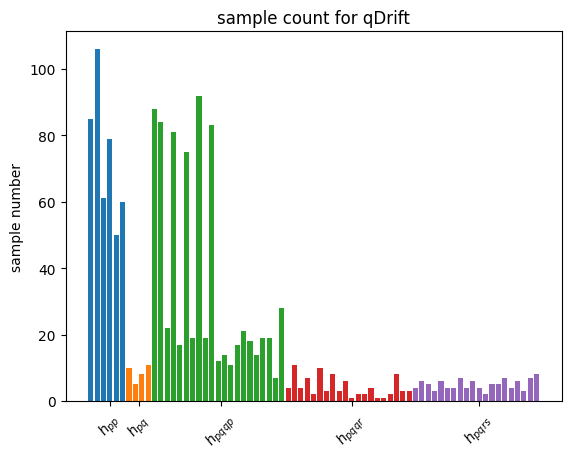
| Intuitively, with the Absolute weights scheme, we are still sampling according to how strong the sub-terms are in the Hamiltonian. This means with N being large, the histogram of Pauli string counts will converge to the one for qDrift(which will ‘drift’ towards particle conserving evolution as well in this sense). We demonstrate this effect with histogram plotted. However, adapt \textit{Mean weights}, Pauli strings with similar physical meaning but opposite signs will dilute the overeall effect. For example, $h_{pqqp}$ in Coulomb group and $h_{pqpq}$ in spin exchange group are in the same sample space as explained above. But the sign will be opposite due to symmetric consideration. $ | h_{pqqp} + h_{pqpq} | \leq | h_{pqqp} | + | h_{pqpq} | $ with the equality achieved when $h_{pqqp} * h_{pqpq} > 0$. |
 However, empirically taken Absolute weights the spectral error is much worse than \textit{mean weights} and even worse than original qDrift, we will use the latter for the rest of the analysis.
Experiment results
In this section we will compare our algorithm with the deterministic approach as well as the randomized ones. But before showing the results, we will elaborate more on how we integrate state-of-art noisy model and relevant mitigation techniques.
Noise model
We categorize the noise into three types:
- Sampling noise: generated by the order of unitaries applied. But we assume that any coherent errors have been removed with the randomised compilation method, leaving only depolarising errors.
- Depokarising noise: we consider stochastic error in each gate which can be simulated by randomly adding a Pauli operator with probability $p$ after each gate – $p$ was chosen to reflect current ion-trap hardware.
- Shot noise: The affect of these is to effectively reduce the amplitude of the measured expectation value by an exponential factor $e^{-t}$, where $t$ is proportional to the depth of the circuit (i.e. number of Pauli exponentials).
We can then assume the simulations run with no noise, but the shot noise $\epsilon_{\text{shot}}$ becomes correlated with the circuit depth[32], causing the number of shots $N_{\text{shot}}$ to scale exponentially with the number of exponentials: \(\epsilon_{\text{shot}} \sim \frac{1}{N_{\text{shot}}^{1/2} e^{-t}} \implies N_{\text{shot}} \sim \frac{1}{\epsilon_{\text{shot}}^2 e^{-2t}}\)
So we will track the spectral error for each of the algorithm at the same circuit depth. And it is not trivial to note that we exchange circuit depth here with the number of Pauli exponentials or Pauli gadgets. This is true provided there is no optimization scheme applied[33,34].
Symmetric protection
We restrict ourselves to the deterministic picture. By exploiting symmetries of the system, that we can substantially reduce the total error $\epsilon$ of the simulation without significantly increasing the gate count[35]. Hamiltonian is invariant under Particle number operator: \([H, \hat{\mathcal{P}}] = 0\)
Because identity operator always commutes with other Pauli strings with same dimension, here $\hat{\mathcal{P}}$ can be simplified to ${exp(−i\phi Z) : \phi \in [0, 2\pi) }$ where $\phi$ is taken randomly between [0, 2] as a multiple of $\pi$. Consider each Trotter step $\mathcal{S}{\delta t} = e^{-iH{eff}t}$ where $H_{eff} = H + \delta H$ the second term being the error. \[e^{-iHt} \implies e^{-iH_{eff}t} = e^{-i( H + \delta H )t}\]
We then extend the original circuit with following protection: \[V = \prod_{k=1}^{N_t} \hat{\mathcal{P}}^{\dag} \mathcal{S}_{\delta t} \hat{\mathcal{P}} = \prod_{k=1}^{N_t} e^{-i( H + \hat{\mathcal{P}}^{\dag} \delta H \hat{\mathcal{P}})t}\]
The second equality is from equation\ref{42}. And the error term will get reduced similar to the averaged distance in random walk. However, we argue that this improvement will not be suitable for randomized approach because there is no fixed known unitary in the circuit, which means the error term is different upon sampling.
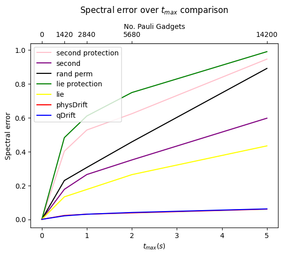
Main result
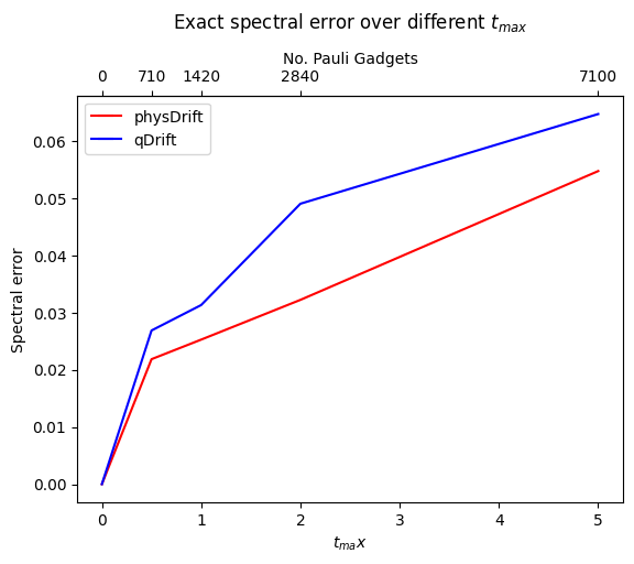
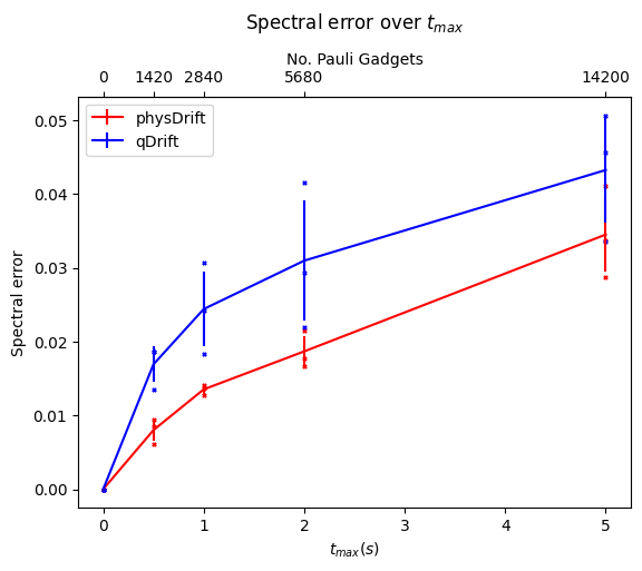
Now we would like to simulate for some time $t_{max}$, and we can only use $N$ exponentials (since the noise on the hardware limits the depth), for which, We assume that typical hardware can use $10^3$ or so CNOT gates. We compared the precision we can get for algorithms mentioned so far without depolarising error first in FIG.\ref{dt8}. Note if not specified the Hamiltonian system is 3-hydrogen chain system.
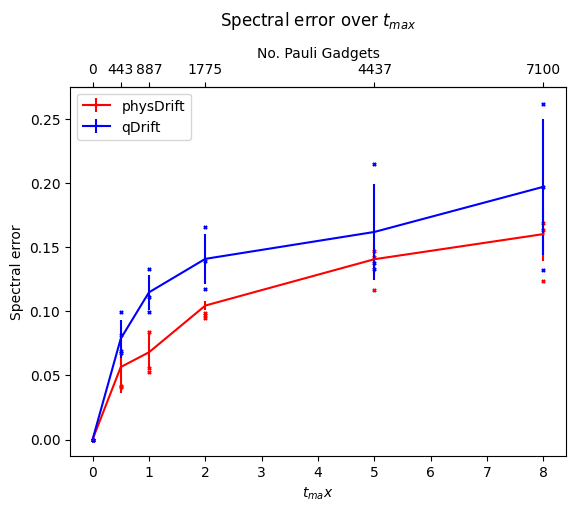
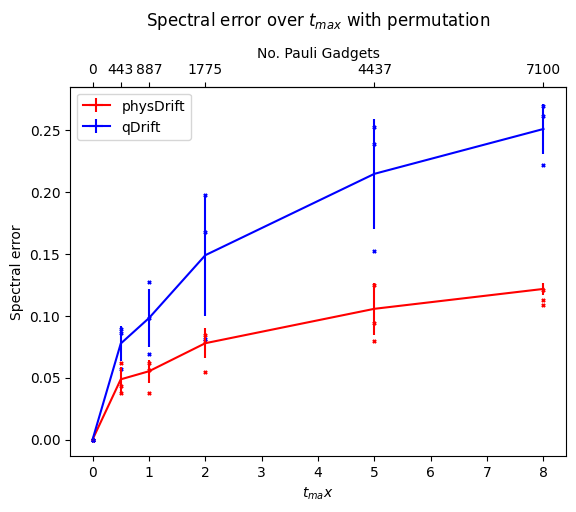
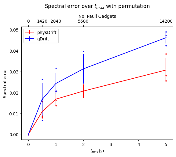
We can see that with our scheme the spectral error is lower and it even performs better when the permutation is taken. However, this has some counter effect on qDrift. To make better analysis, we next move on comparing the exact evolution at the time where each whole group in the physDrift is applied with the simulation
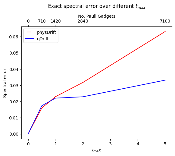
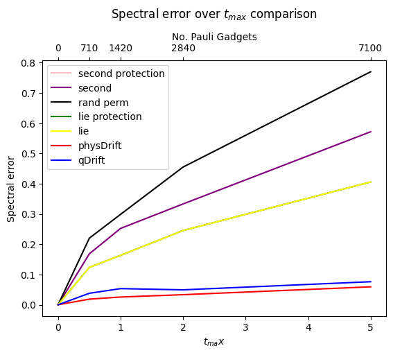
The result has been improved for the permuted one. In contrast the one with just averaging the raw experimental result does not predict the structure of evolution as accurate as qDrift. Adding in other algorithms in FIG.\ref{spec}

With the following lemma we explain why the empirical result for physDrift is better than qDrift.
Lemma 3
Given a pool of $\mathcal{R}(\mathcal{L}1,\mathcal{L}_2,\dots,\mathcal{L}{L})$ to implement random samples of unitary, the spectral error is always greater than or equal to the protocol with a pool of $\hat{\mathcal{R}}(\mathcal{L}1,\mathcal{L}_2,\dots,\mathcal{L}_i+\mathcal{L}_j,\dots \mathcal{L}{\hat{L}})$ where $\hat{L} \leq L$. ***
Proof
By Equation(31), \(\Vert \mathcal{U}_N-\mathcal{V}_N \Vert_\diamondsuit = \left\Vert \sum_{n=2}^\infty \frac{t^n\mathcal{L}^n}{n!N^n}-\sum_{j}\frac{h_j}{\lambda} \sum_{n=2}^\infty \frac{\lambda^n \tau^n \mathcal{L}_j^n}{n!N^n} \right\Vert_\diamondsuit\) \(\leq \sum_{n=2}^\infty \frac{t^n \left\Vert \mathcal{L}^n \right\Vert_\diamondsuit}{n!N^n}+\sum_{j}\frac{h_j}{\lambda} \sum_{n=2}^\infty \frac{ \lambda^n \tau^n \left\Vert \mathcal{L}_j^n \right\Vert_\diamondsuit}{n!N^n}\) where the first order cancels with the choice of $\tau = \lambda t / N$. Looking at the second term, we know from subadditivity of diamond norm $\Vert A + B \Vert_\diamondsuit \leq \Vert A \Vert_\diamondsuit + \Vert B \Vert_\diamondsuit$ that $\Vert \mathcal{L}1^n \Vert\diamondsuit + \Vert \mathcal{L}2^n \Vert\diamondsuit + \dots \Vert (\mathcal{L}i+\mathcal{L}_j)^n \Vert\diamondsuit + \dots + \Vert \mathcal{L}{\hat{L}}^n \Vert\diamondsuit = \sum_j^{\hat{L}} \Vert \mathcal{L}{\hat{j}}^n \Vert\diamondsuit \leq \Vert \mathcal{L}1^n \Vert\diamondsuit + \Vert \mathcal{L}2^n \Vert\diamondsuit + \dots + \Vert \mathcal{L}{L}^n \Vert\diamondsuit = \sum_j^L \Vert \mathcal{L}j^n \Vert\diamondsuit$. This means that by combining more commuting terms together the theoretical bound will become tighter. ***
Besides particle number, we also track the expectation of the $\langle H \rangle$, which, under exact evolution, should be conserved. So it’s easy to see how the error fluctuations.
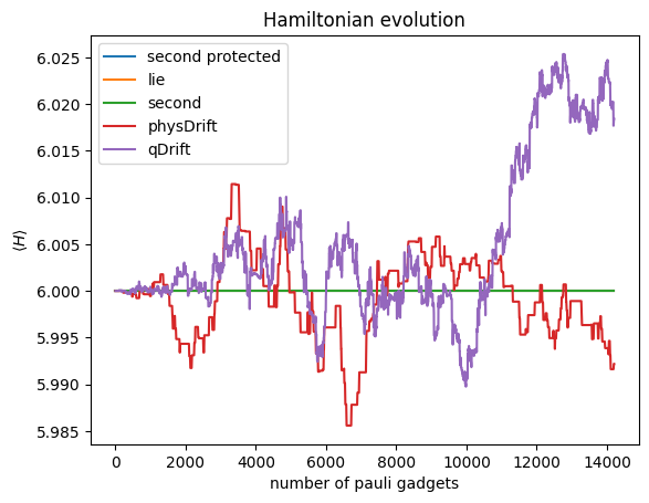
As we can see the fluctuation of physDrift concentrates around the expected energy while the one for qDrift overshoots after a while. This mean physDrift actually has more tendency to stay in physical space $\mathcal{H}_{phys}$.
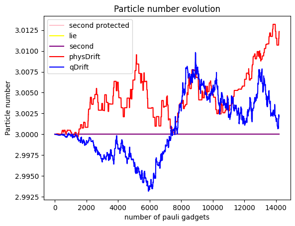
To our disappointment, it seems that qDrift does slight better again than physDrift. What about electron counts at a particular moelcular orbit?
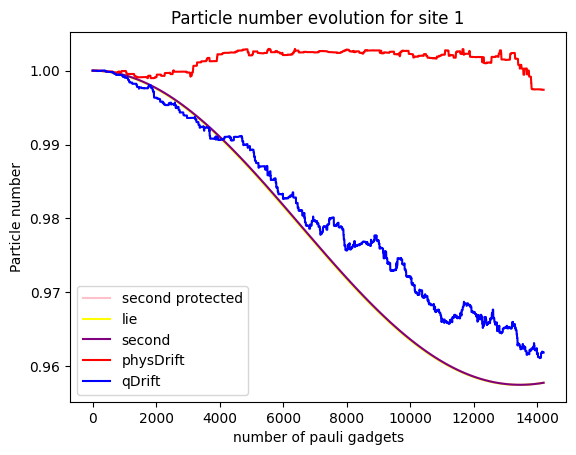
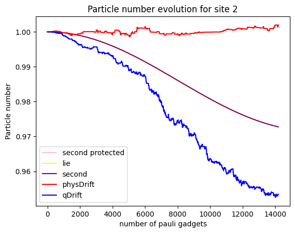
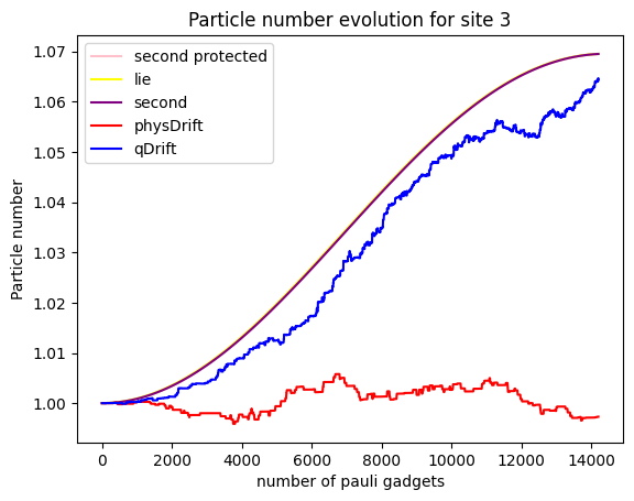 It seems that the
Note that generally, the simulation of an expectation value can be good, but the simulation of the state itself might be bad. But it is not true the other way around.
Noisy Simulation
Now we add some depolarising error with strength parameter around 0.1\%\cite{error}
acknowledgments
We wish to acknowledge the support of Dr.Alex Thom for helpful discussion as well as suggestions on the relevant topics.
[1] R. P. Feynman, Int. j. Theor. phys 21 (1982).
[2] S. Lloyd, Universal quantum simulators, Science 273, 1073 (1996).
[3] N. Hatano and M. Suzuki, Finding exponential prod- uct formulas of higher orders, in Quantum annealing and other optimization methods (Springer, 2005) pp. 37–68.
[4] A. M. Childs and N. Wiebe, Hamiltonian simulation using linear combinations of unitary operations, arXiv preprint arXiv:1202.5822 (2012).
[5] G. H. Low and I. L. Chuang, Optimal hamiltonian sim- ulation by quantum signal processing, Physical review letters 118, 010501 (2017).
[6] D. W. Berry, A. M. Childs, R. Cleve, R. Kothari, and R. D. Somma, Simulating hamiltonian dynamics with a truncated taylor series, Physical review letters 114, 090502 (2015).
[7] A. M. Childs, Y. Su, M. C. Tran, N. Wiebe, and S. Zhu, Theory of trotter error with commutator scaling, Physi- cal Review X 11, 011020 (2021).
[8] A. M. Childs and Y. Su, Nearly optimal lattice simulation by product formulas, Physical review letters 123, 050503 (2019).
[9] R. Barends, L. Lamata, J. Kelly, L. García-Álvarez, A. G. Fowler, A. Megrant, E. Jeffrey, T. C. White, D. Sank, J. Y. Mutus, et al., Digital quantum simula- tion of fermionic models with a superconducting circuit, Nature communications 6, 7654 (2015).
[10] K. R. Brown, R. J. Clark, and I. L. Chuang, Limitations of quantum simulation examined by simulating a pairing hamiltonian using nuclear magnetic resonance, Physical review letters 97, 050504 (2006).
[11] Z.-J. Zhang, J. Sun, X. Yuan, and M.-H. Yung, Low- depth hamiltonian simulation by an adaptive product formula, Physical Review Letters 130, 040601 (2023).
[12] H. Yoshida, Construction of higher order symplectic in- tegrators, Physics letters A 150, 262 (1990).
[13] T. Barthel and Y. Zhang, Optimized lie–trotter–suzuki decompositions for two and three non-commuting terms, Annals of Physics 418, 168165 (2020).
[14] G. H. Low, V. Kliuchnikov, and N. Wiebe, Well- conditioned multiproduct hamiltonian simulation, arXiv preprint arXiv:1907.11679 (2019).
[15] B. D. Jones, D. R. White, G. O. O’Brien, J. A. Clark, and E. T. Campbell, Optimising trotter-suzuki decompo- sitions for quantum simulation using evolutionary strate- gies, in Proceedings of the Genetic and Evolutionary Computation Conference (2019) pp. 1223–1231.
[16] A. M. Childs, A. Ostrander, and Y. Su, Faster quantum simulation by randomization, Quantum 3, 182 (2019).
[17] E. Campbell, Shorter gate sequences for quantum com- puting by mixing unitaries, Physical Review A 95, 042306 (2017).
[18] M. B. Hastings, Turning gate synthesis errors into inco- herent errors, arXiv preprint arXiv:1612.01011 (2016).
[19] E. Campbell, Random compiler for fast hamiltonian sim- ulation, Physical review letters 123, 070503 (2019).
[20] P. Jordan and E. P. Wigner, Über das paulische äquiv- alenzverbot (Springer, 1993).
[21] J. T. Seeley, M. J. Richard, and P. J. Love, The bravyi- kitaev transformation for quantum computation of elec- tronic structure, The Journal of chemical physics 137 (2012).
[22] S. Bravyi, J. M. Gambetta, A. Mezzacapo, and K. Temme, Tapering off qubits to simulate fermionic hamiltonians, arXiv preprint arXiv:1701.08213 (2017).
[23] Q. Zhao and X. Yuan, Exploiting anticommutation in hamiltonian simulation, Quantum 5, 534 (2021).
[24] K. Kraus, General state changes in quantum theory., Czechoslovak Journal of Physics, Vol. B 11, 546 (1961).
[25] C. Yi and E. Crosson, Spectral analysis of product formu- las for quantum simulation, npj Quantum Information 8, 37 (2022).
[26] C.-F. Chen, H.-Y. Huang, R. Kueng, and J. A. Tropp, Concentration for random product formulas, PRX Quan- tum 2, 040305 (2021).
[27] O. Kiss, M. Grossi, and A. Roggero, Importance sam- pling for stochastic quantum simulations, Quantum 7, 977 (2023).
[28] S. T. Tokdar and R. E. Kass, Importance sampling: a review, Wiley Interdisciplinary Reviews: Computational Statistics 2, 54 (2010).
[29] Y. Ouyang, D. R. White, and E. T. Campbell, Compi- lation by stochastic hamiltonian sparsification, Quantum 4, 235 (2020).
[30] J. J. Wallman and J. Emerson, Noise tailoring for scalable quantum computation via randomized compiling, Physi- cal Review A 94, 052325 (2016).
[31] K. Gui, T. Tomesh, P. Gokhale, Y. Shi, F. T. Chong, M. Martonosi, and M. Suchara, Term grouping and trav- elling salesperson for digital quantum simulation (2021), arXiv:2001.05983 [quant-ph].
[32] E. Granet and H. Dreyer, Continuous hamiltonian dy- namics on noisy digital quantum computers without trot- ter error (2023), arXiv:2308.03694 [quant-ph].
[33] A. Kissinger and J. van de Wetering, Reducing the num- ber of non-clifford gates in quantum circuits, Physical Review A 102, 10.1103/physreva.102.022406 (2020).
[34] M. B. Hastings, D. Wecker, B. Bauer, and M. Troyer, Improving quantum algorithms for quantum chemistry (2014), arXiv:1403.1539 [quant-ph].
[35] M. C. Tran, Y. Su, D. Carney, and J. M. Taylor, Faster digital quantum simulation by symmetry protec- tion, PRX Quantum 2, 10.1103/prxquantum.2.010323 (2021).
[36] F. C. . P. R. Chen, YT., Low-rank density-matrix evo- lution for noisy quantum circuits, npj Quantum Inf 7 61 (2021).
[37] J. Watrous, The Theory of Quantum Information (Cam- bridge University Press, 2018).
[38] A. K. D. Aharonov and N. Nisan, Quantum circuits with mixed states. In Proceedings of the Thirtieth Annual ACM Symposium on Theory of Computing (Association for Computing Machinery, 1998).
[39] A. M. Childs, D. Maslov, Y. Nam, N. J. Ross, and Y. Su, Toward the first quantum simulation with quan- tum speedup, Proceedings of the National Academy of Sciences 115, 9456 (2018).