Deep learning in MRI
Supervisor: Prof. Chris Rogers (Fellow of Peterhouse, Department of Clinical Neurosciences)
Use of deep learning to accelerate parallel transmit pulse design
We want to develop a neural network (NN) based design to make the current approach, either through rodrigue’s rotation or the quaternion way, of designing pulse faster. Because of universal approximation theorem, a continuous function like rotational function in our case can be generated with NN and it should be faster than direct computation of the function.
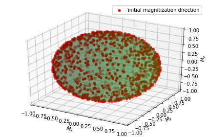
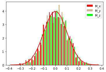
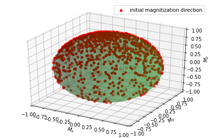
To simplify the task, we first concentrate on setting the initial magnetization direction as the only changing variables, which will be fed into the vanilla neural network. InVanilla_neural_network, we sampled 1000 random points on the surface of the unit sphere (keep normalisation) with Gaussian distribution.
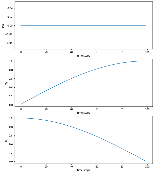
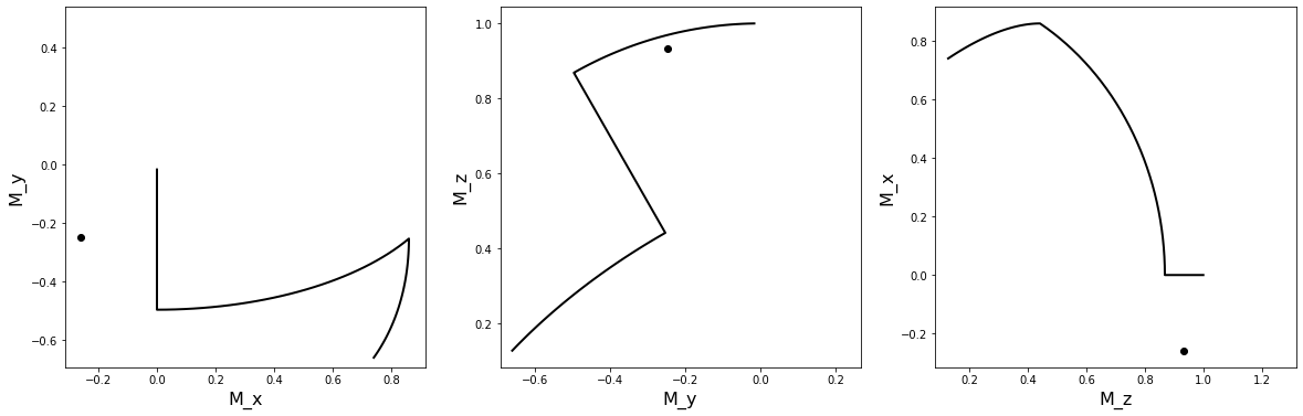
With the gradient value set to 0, b0 to 0 and b1 offset to 250Hz as default, we plotted the rotation based on the quaternion approach (Blochsim). Here the initial direction is [0,0,1] and with 90 degree rotation the final direction sits on [0,1,0] (sign might differ because of convention).
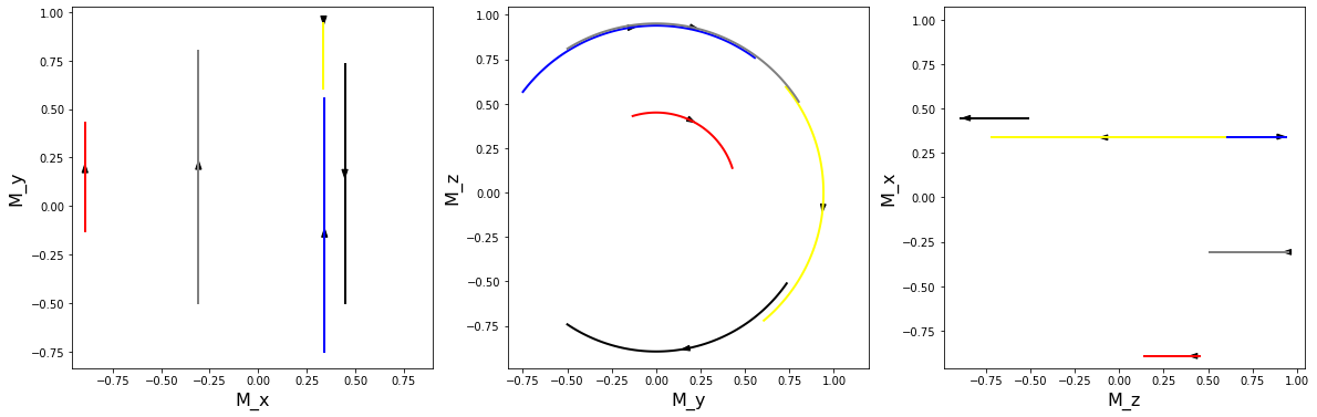
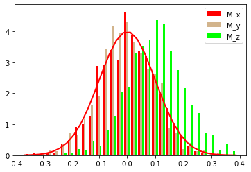
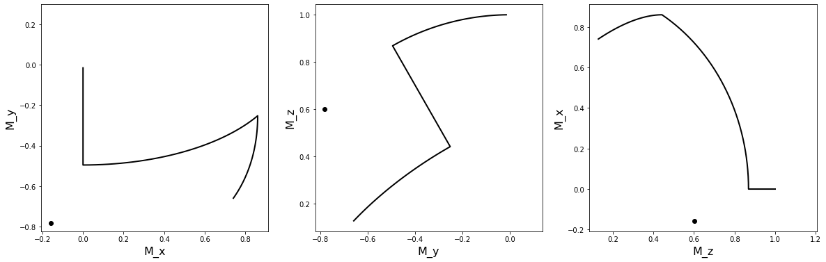
Then we made plots of the magnetization viewed sideways from 2 dimensional planes.
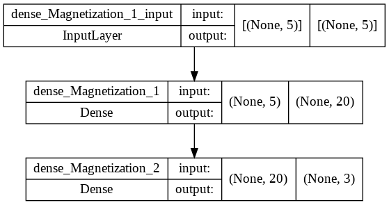
So all the functions are working and we began to build the architecture of our neural network. To start easy, we used the simplest one shown below:

So the input is a 3 dimensional parameter with x, y, z direction components. None value here is the number of samples we put in. There is only one hidden layer which takes the input and ‘distributes’ them according to some weights to 20 nodes. In the output layer we then have 3 rotated directions.
To easily debug the training, we first added a bias to the z direction so that the points only concentrate on the top of the unit sphere.
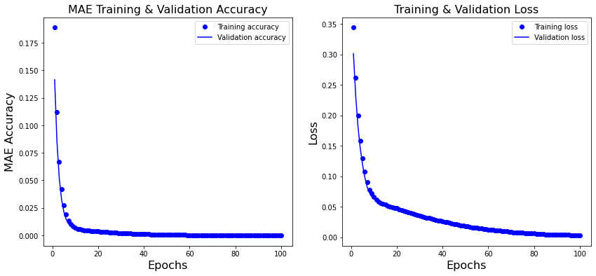
Then we started to train the NN and below are the plots of the predictions as well as the loss.

Predicted: [0.47880924 -0.8103403 -0.33777267]
original: [0.48110492 -0.80970572 -0.33602784]
Predicted: [-0.20483616 0.50461364 0.83869374]
original: [-0.20033752 0.50677293 0.83847843]
Predicted: [0.1408676 0.72912085 0.66973066]
original: [0.15265431 0.73098737 0.66509709]
While training the model we will save the trained weights for later use.
We went on with an additional parameter: b0 offset. It’s clear to get a visualisation of the effect of this offset from Keeler’s book:
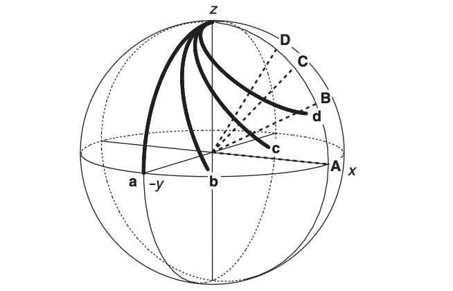
Path a is for the on-resonance case. The effective field lies along x and is indicated by the dashed line A. Path b is for the case where the offset is half the RF field strength; the effective field is marked B. Paths c and d are for offsets equal to and 1.5 times the RF field strength, respectively. The effective field directions are labelled C and D.
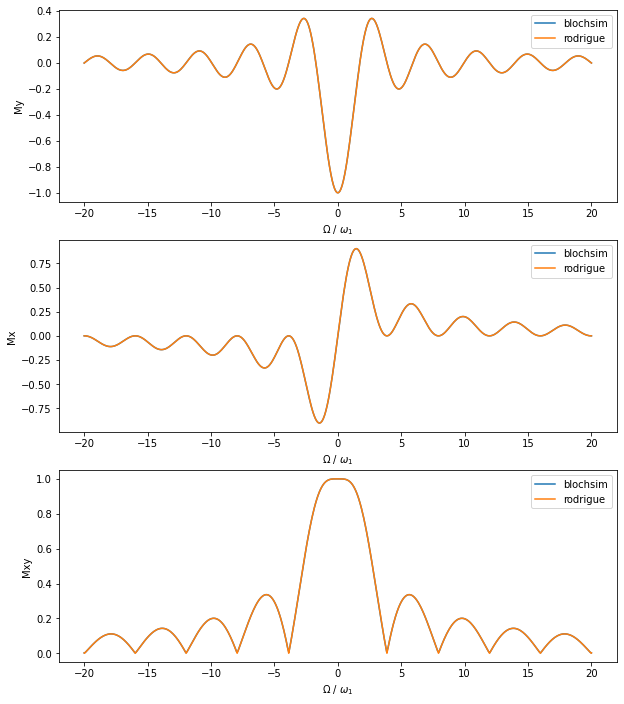
To demonstrate how close the rotational function (rodrigue) used above and Blochsim, we made plots of both cases with respect to the offset see below:
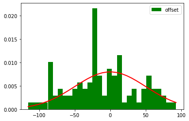
Similarly, we sampled with normal distribution the offset around 50Hz. First we construct the NN with rodrigue’s approach.
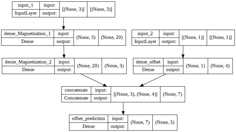
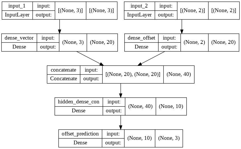
We refer to the following architecture as ‘2-stream’ because of the way we feed in parameters: concatenating the left (initial magnetization) and right (b0 offset) from two different hidden layers, one with 20 nodes and the other 4 nodes and get output from the concatenation layer.
The result is quite good actually, with total training time 322.8357243537903 and loss=0.0453, mse=0.00429. (below is prediction from [0.7, 0.7, 0.5] and offset 0)

predicted: [0.99999666 -0.00114888 0.00232671]
original: [1. 0. 0.]
predicted: [-0.00322477 0.00378172 0.99998766]
original: [0.000000e+00 -6.123234e-17 1.000000e+00]
predicted: [0.00864881 0.999947 -0.00558268]
original: [0.000000e+00 1.000000e+00 6.123234e-17]
With the quaternion approach we have loss=0.347, mse=0.227 and 322.0919027328491.
(below is prediction from [0, 0, 1] and offset 0)
predicted: [-0.99005747 0.07547599 0.11869986]
original: [1. 0. 0.]
predicted: [-0.41254485 0.9078387 0.07507148]
original: [0.00000000e+00 -2.08091499e-04 -9.99999978e-01]
predicted: [0.01036049 0.00709057 0.99992114]
original: [0.00000000e+00 -9.99999978e-01 2.08091499e-04]
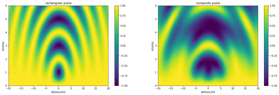
Next we experimented with Composite pulse, with which, as we can see below, the first blob (rotation) region has more tolerance than normal rectangular pulse.
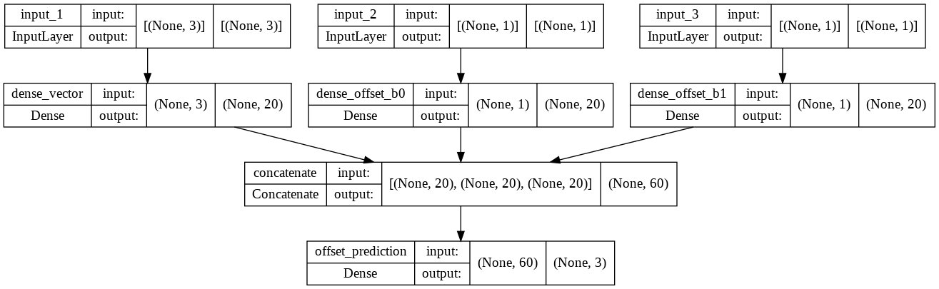
For the model architecture, we have 3 different approach:
3 stream with input streams: initial magnetization, b0 offset and b1 offset
predicted: [-0.9189578 0.12260745 0.37481192]
original: [0.50915963 0.42637612 -0.7476362]
predicted: [-0.9189578 0.12260745 0.37481192]
original: [0.43806533 0.61934441 0.65154529]
predicted: [-0.9189578 0.12260745 0.37481192]
original: [0.74084765 -0.65925406 0.12856457]
2 streamwith input streams: initial magnetization, b0 offset and b1 offset combined
predicted: [0.19750698 0.5291543 -0.82521915]
original: [0.47361248 0.52286026 -0.04804545]
predicted: [0.19750698 0.5291543 -0.82521915]
original: [0.43806533 0.61934441 0.65154529]
predicted: [0.19750698 0.5291543 -0.82521915]
original: [0.74084765 -0.65925406 0.12856457]
5 dimension parameters with the original architecture plus one more hidden layer
predicted: [-0.72018874 -0.6089137 -0.33249408]
original: [0.50915963 0.42637612 -0.7476362]
predicted: [0.1996805 0.41469178 0.8877829]
original: [0.43806533 0.61934441 0.65154529]
predicted: [-0.04655632 0.8061741 -0.589844]
original: [0.74084765 -0.65925406 0.12856457]
Next we restrict the initial vector on direction [0,0,1]:
5d model
predicted: [-0.13396332 -0.59929323 0.7892411]
original: [0. -0.58771791 0.80906592]
predicted: [0.04798383 0.0153396 0.9987303]
original: [0.19769059 0.00778452 0.98023356]
predicted: [0.08250432 -0.00681832 0.9965674]
original: [2.05595885e-04 -5.36070276e-03 9.99985610e-01]
Stream
predicted: [-0.26739812 -0.586575 0.764479]
original: [0. -0.58771791 0.80906592]
predicted: [0.09361884 -0.01209054 0.9955347]
original: [0.19769059 0.00778452 0.98023356]
predicted: [0.0616199 0.01683904 0.99795765]
original: [2.05595885e-04 -5.36070276e-03 9.99985610e-01]
Relevant code can be found here