Quantum simulation on NV center
Advisor: Dr. Helena Knowles (Assistant Professor Royal Society University Research Fellow, Cavendish)
Simulations on NV centers
Some of the code were inspired by
- https://github.com/lukastk/nv-centre-spectrum-simulator
- https://github.com/sashankkaushik/qutip_NV_Dynamics
NV center simulation
Negatively charged nitrogen-vacancy centers (NV) in diamond have emerged as promising platforms for quantum information processing and for a wide range of applications in quantum sensing [1]. NV centers with long spin coherence make it an excellent candidate for quantum technologies. Many experiments have been conducted to measure the dephasing time T2 and how to enhance it in the NV system. This code repo is used to simulate the physical situation and make comparison with the real data to help improve the technique.
Isolated NV centers
For a typical NV center we can visualize it as following
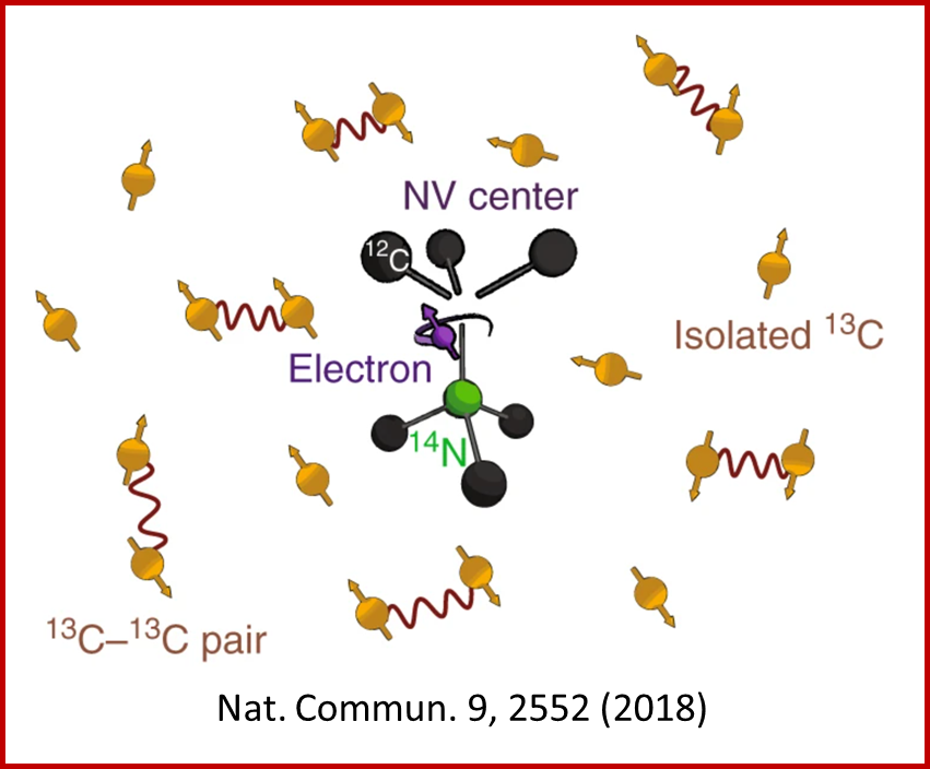
where it consists of a nitrogen center with electon triplet and it can interact with the $C^{13}$ as well as other NV centers in the environment.
But here we consider two isolated and simplified NV centers without interaction with the environment. In this case we care about the NV-NV dipole interaction.
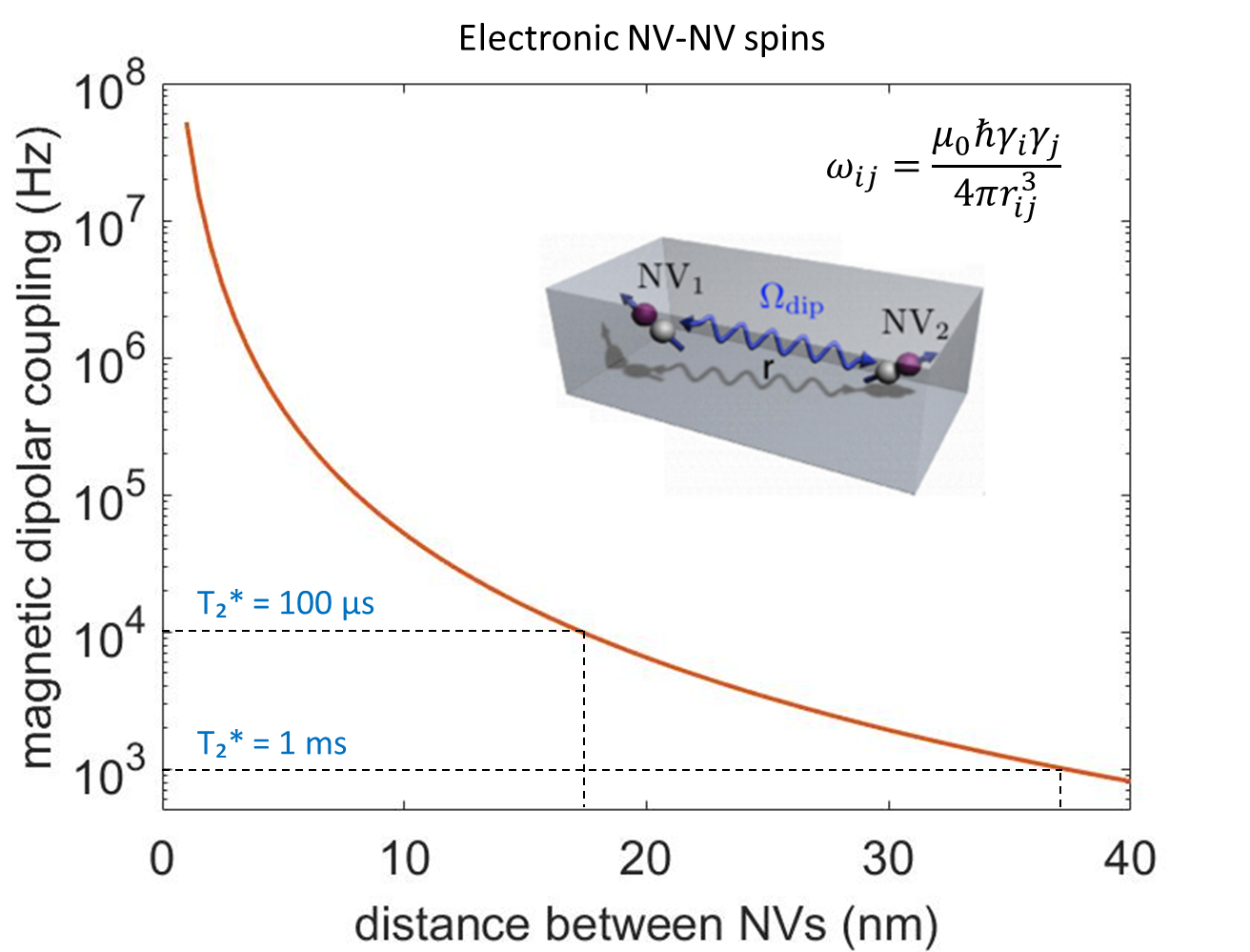
the parameter we are interested in is the magnetic dipolar coupling $\omega$ and the $\gamma_i$, $\gamma_j$ in the formula is gyromagnetic ratio of the ‘i’ and ‘j’ spin (rad/(s.T)).
For an electron the value is $\gamma_e$ = $1.760859644*10^{11}$ (rad/(s.T)).
we used MATLAB to simulate the coupling coefficient.
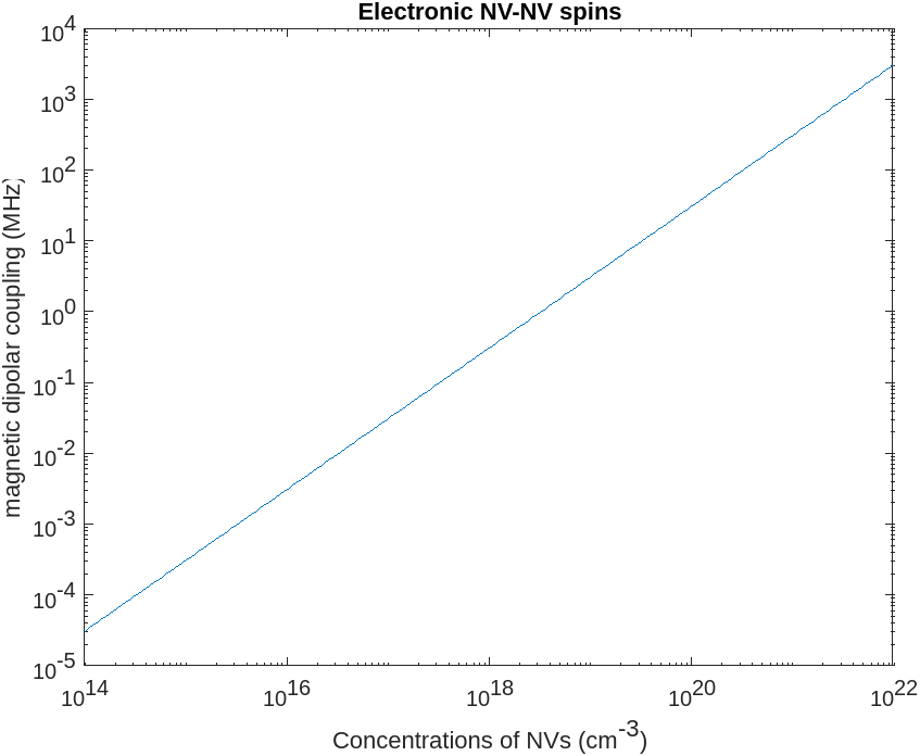
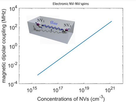
we also want to simulate multiple coupling constant. For example, place each NV centers on a corner of the octahedron and see how the coupling changes. We can control the distance between NV centers by change the concentration of the NV centers, under the assumptions that NVs are uniformly distributed.
The distribution of molecules in solution is not uniform but has a distribution. The nearst neighbor distance from one molecule to another has been worked out by [3], r = 0.55396*$n^{\frac{1}{3}}$, where n is the concentration of NVs.
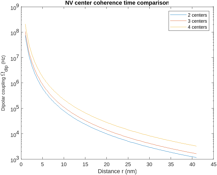
Then to get a more realistic picture, we simulated a spectrum of coupling schemes and record the occurence to see the distribution of the possible configuration. To model this, consider a fixed concenration of NV centers inside a cube of given size. And because NV centers can point towards one of the 4 possible orientations of the lattice tetrahedron, which affects the coupling. We simulate the effect by taking a random distribution of the direction.
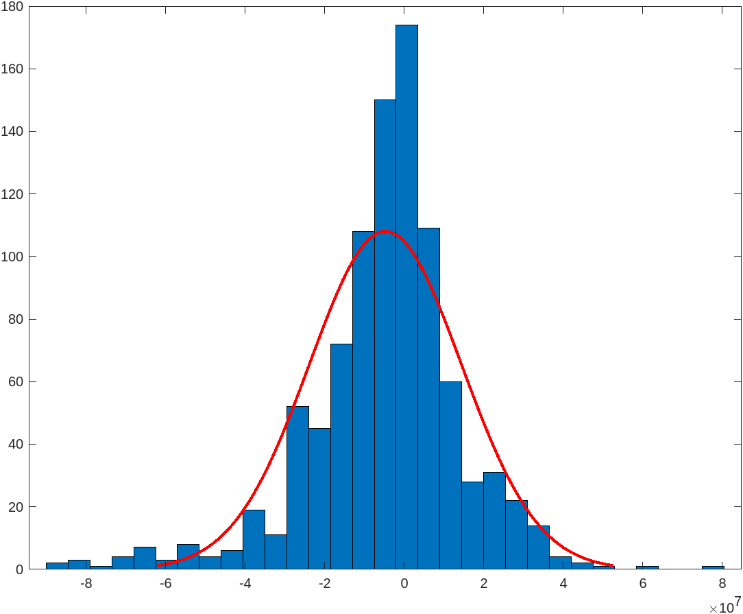
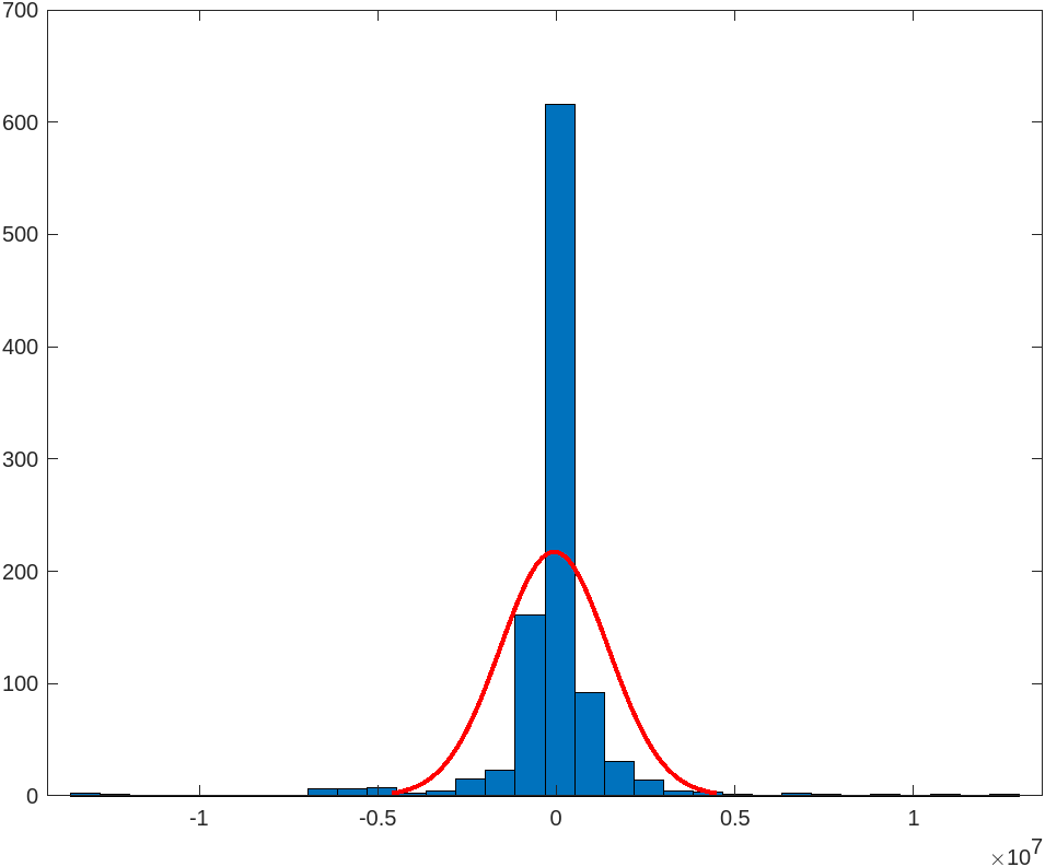
We changed the concentration above.
From classical to quantum
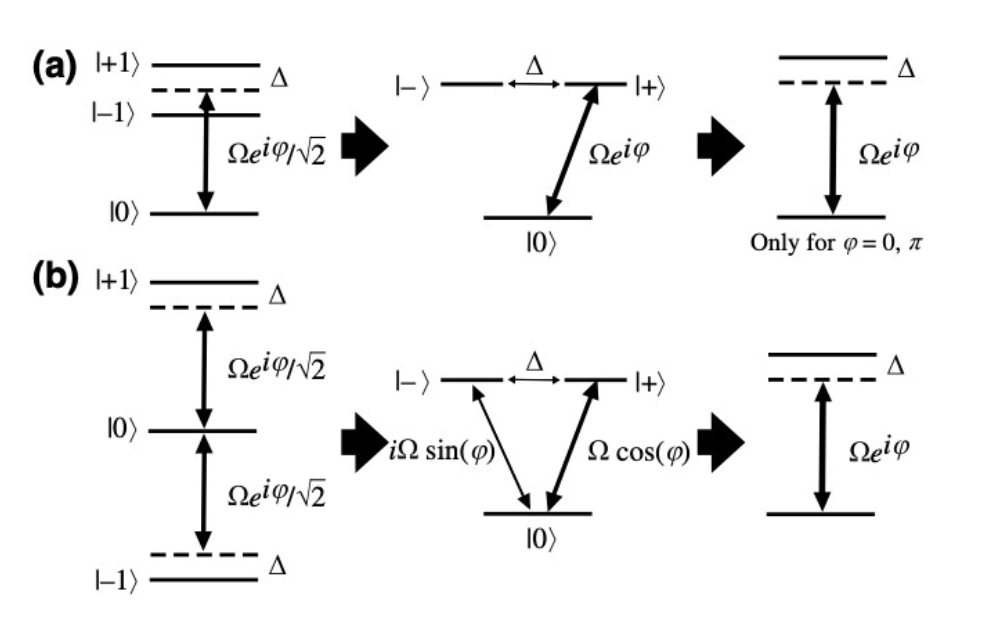
What we talked before involves classical interactions only. However, to account for quantum interaction we need to change simple multiplication to tensor product.
The dipole dipole interaction is then:
$\displaystyle V(r) = \frac{1}{r^3} \frac{3(\vec{\sigma_1}\cdot\vec{r_1})(\vec{\sigma_2}\cdot\vec{r_2})-r^2(\vec{\sigma_1}\cdot\vec{\sigma_2})}{r^2}$
for spin-1/2 particles we have,
$\displaystyle \vec{\sigma} = \left(\sigma_x, \sigma_y, \sigma_z \right) = \left( \begin{pmatrix} 0 & 1 \ 1 & 0 \end{pmatrix}, \begin{pmatrix} 0 & i \ -i & 0 \end{pmatrix}, \begin{pmatrix} 1 & 0 \ 0 & -1 \end{pmatrix} \right)$
where $\vec{\sigma_1}\cdot\vec{r_1}$, $\vec{\sigma_2}\cdot\vec{r_2}$ is $\sigma_1(i) \sigma_2(j) r_i r_j$ and $\sigma_1(i) \sigma_2(j) = \sigma_1(i) \otimes \sigma_2(j)$
for example, in matrix form
$\sigma_1(x) \otimes \sigma_2(y)$ = $\begin{pmatrix} 0 & \sigma_y \ \sigma_y & 0 \end{pmatrix}$ = $\begin{pmatrix} 0 & 0 & 0 & i \ 0 & 0 & -i & 0 \ 0 & i & 0 & 0 \ -i & 0 & 0 & 0 \end{pmatrix}$
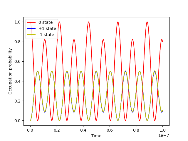
What we eventually want is quantum control over different states. This leads to the introduction to rabi oscillation [2].
Rabi oscillation is a phenomenon that occurs in quantum systems when they are subjected to an oscillating electromagnetic field at a resonant frequency. It is named after physicist Isidor Rabi, who first observed this effect in the 1930s.
| In simple terms, Rabi oscillation describes the periodic and reversible exchange of energy between a two-level quantum system and an external field. The two levels of the system can be represented as the ground state ( | 0⟩) and an excited state ( | 1⟩). When the system is in the ground state, the external field can induce transitions to the excited state, and vice versa. |
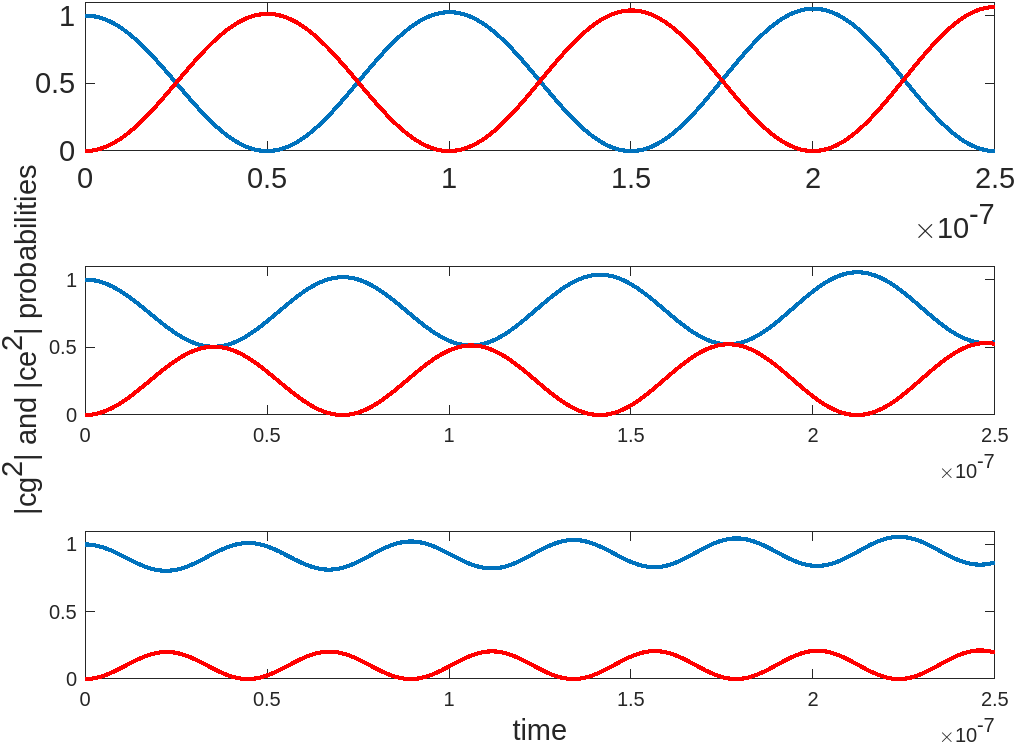
The dynamics of Rabi oscillation can be described by the Schrödinger equation in quantum mechanics or the Bloch equations in the context of spin systems. The amplitude and frequency of the oscillation depend on the strength and duration of the applied field. The Rabi frequency (Ω) represents the strength of the coupling between the system and the external field.
Detuning refers to the situation when the frequency of the applied field deviates from the resonant frequency of the quantum system. In other words, the external field is not perfectly matched to the energy difference between the two levels. When detuning occurs, the system still undergoes oscillations, but the amplitude and frequency of the oscillation change.
Above we used qutip to simulate the probability for the atom being in one particular state.
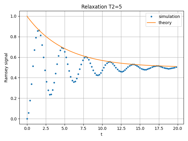
Qutip is a very powerful package. We can have a brief look at the simulation for T2 relaxation,arising from the interactions between the electronic spin of the NV center and its surrounding environment, which can include nuclear spins, lattice vibrations, and magnetic field fluctuations. These interactions cause the quantum phase information of the spin state to become randomized, leading to a loss of coherence.
import numpy as np
import matplotlib.pyplot as plt
from qutip.qip.device import Processor
from qutip.operators import sigmaz, destroy
from qutip.qip.operations import snot
from qutip.states import basis

a = destroy(2)
Hadamard = snot()
plus_state = (basis(2,1) + basis(2,0)).unit()
tlist = np.arange(0.00, 20.2, 0.2)

T2 = 5
processor = Processor(1, t2=T2)
processor.add_control(sigmaz())
processor.pulses[0].coeff = np.ones(len(tlist))
processor.pulses[0].tlist = tlist
result = processor.run_state(
    plus_state, e_ops=[a.dag()*a, Hadamard*a.dag()*a*Hadamard])

fig, ax = plt.subplots()
# detail about length of tlist needs to be fixed
ax.plot(tlist[:-1], result.expect[1][:-1], '.', label="simulation")
ax.plot(tlist[:-1], np.exp(-1./T2*tlist[:-1])*0.5 + 0.5, label="theory")
ax.set_xlabel("t")
ax.set_ylabel("Ramsey signal")
ax.legend()
ax.set_title("Relaxation T2=5")
ax.grid()
fig.tight_layout()
fig.show()
Detuning can be used to control and manipulate quantum systems. By adjusting the detuning, one can influence the dynamics of Rabi oscillations and achieve specific quantum operations, such as population transfer between the levels or coherent control of qubits in quantum computing.
For example: \[H=\Delta(t)\sigma_z+\omega_R\sigma_x=\left( \begin{array}{ccc} \Delta(t) & \omega_R \\ \omega_R & -\Delta(t) \\ \end{array} \right)\]
where $\Delta(t)$ is detuning and $\omega_R$ Rabi frequency. By changing the pulse duration we can get different quantum states (gates).
Another way to simplify rabi simulation is to consider the Interaction Picture and Rotation Wave Approximation (RWA) [3]
 \[\hat{H}=-\frac{\Delta}{2}\sigma_z+\frac{\omega_1}{2}\sigma_x \\\overset{\text{$\Delta=\omega_0-\omega$}}{\xlongequal{\quad\quad\quad}}\frac{1}{2} \begin{pmatrix} \omega-\omega_0 & \omega_1 \\ \omega_1 & \omega_0-\omega \end{pmatrix} \\=\frac{1}{2} \begin{pmatrix} \Delta & \omega_1 \\ \omega_1 & \Delta \end{pmatrix}\]
where we have ignored the higher frequency order terms.
Microwave frequency sweep
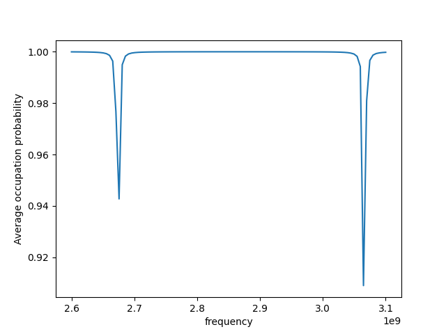
Next, we tried to find the Dzfs value at 2.87GHz from a microwave sweep.
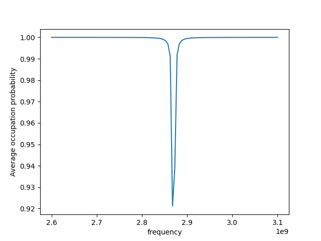
With a magnetic field and external decoherence factor applied, the tip splited and shifted at a different value as below:
Data matching
With the above tested, we switched back to MATLAB with the algorithm used in qutip. Now experiementally we have obtained some pulse data and we fitted as well as optimized them as following:
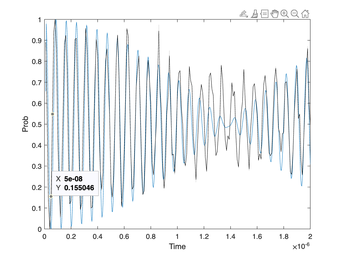
Rabi oscillation fit. Although we have some flctuations around the dip, we can see on a large scale, the simulation matches pretty well.
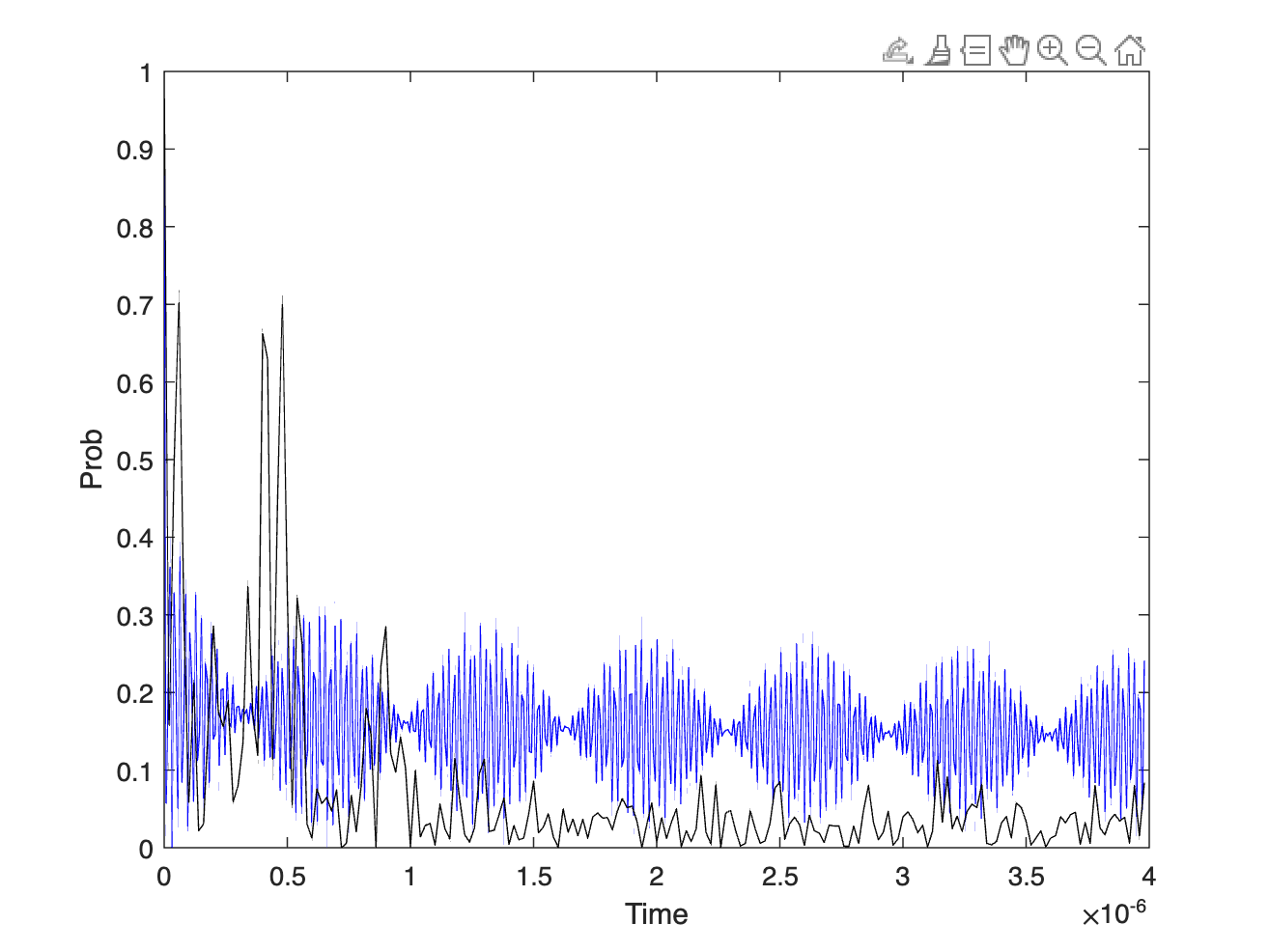
This is the ramsey pulse fit. A Ramsey pulse [4] is based on the principle of quantum interference. It exploits the property of superposition, where a quantum system can exist in multiple states simultaneously. In the case of a qubit, it can be in a superposition of both the 0 and 1 states.
To understand the Ramsey pulse, let’s consider a simplified example with a single qubit. The qubit is first put into a superposition of both the 0 and 1 states by applying a Hadamard gate (H gate) to it. The H gate rotates the qubit state by 90 degrees around the Bloch sphere, a geometric representation of the qubit states.
| After the H gate, the qubit is in a superposition of | 0⟩ and | 1⟩, represented as ( | 0⟩ + | 1⟩)/√2. This superposition is achieved by splitting the qubit’s probability amplitude equally between the 0 and 1 states. |
Next, a phase shift is applied to the qubit. This phase shift is typically implemented by applying a microwave pulse for a specific duration, which effectively rotates the qubit’s state around the z-axis of the Bloch sphere. The duration of this phase shift pulse is known as the Ramsey time.
| The phase shift introduces a relative phase between the two superposed states. The resulting state becomes ( | 0⟩ + e^(iθ) | 1⟩)/√2, where θ is the phase angle determined by the duration of the phase shift pulse. |
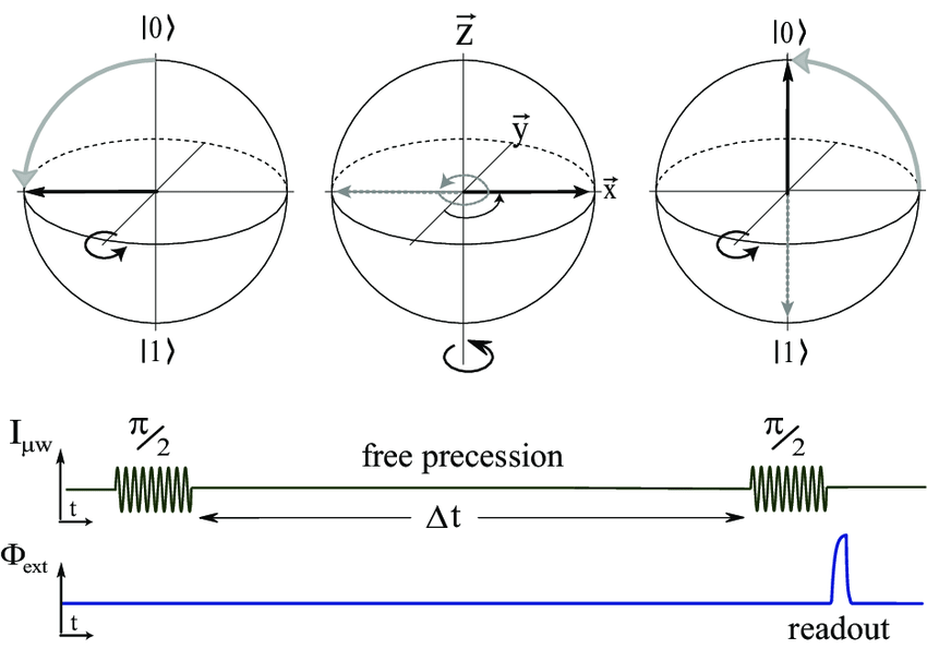
Finally, another H gate is applied to the qubit. This second H gate effectively rotates the qubit’s state by another 90 degrees, bringing the relative phase introduced by the Ramsey time into an observable effect.
The final state of the qubit after the second H gate is measured. The relative phase between the two superposed states causes the probability amplitudes to interfere constructively or destructively, resulting in an observable interference pattern during measurement. By varying the duration of the Ramsey time, one can observe the oscillatory behavior of the interference pattern.
Reference
[1] Hollendonner, M., et al. “Quantum sensing of electric field distributions of liquid electrolytes with NV-centers in nanodiamonds.” arXiv preprint arXiv:2301.04427 (2023). [2] Jacques, V., et al. “Dynamic polarization of single nuclear spins by optical pumping of NV color centers in diamond at room temperature.” arXiv preprint arXiv:0808.0154 (2008). [3] PHYSICAL REVIEW APPLIED 17, 044028 (2022) Zero- and Low-Field Sensing with Nitrogen-Vacancy Centers [4] Hong, Sungkun, et al. “Nanoscale magnetometry with NV centers in diamond.” MRS bulletin 38.2 (2013): 155-161.
Relevant code can be found here